Case Study: How Does a Bike-Share Navigate Speedy Success?
Table of Contents
Scenario
You are a junior data analyst working in the marketing analyst team at Cyclistic, a bike-share company in Chicago. The director of marketing believes the company’s future success depends on maximizing the number of annual memberships. Therefore, your team wants to understand how casual riders and annual members use Cyclistic bikes differently. From these insights, your team will design a new marketing strategy to convert casual riders into annual members. But first, Cyclistic executives must approve your ecommendations, so they must be backed up with compelling data insights and professional data visualizations.
Ask Phase
Guiding questions
-
What is the problem you are trying to solve?
-
How do annual members and casual riders use Cyclistic bikes differently?
-
Why would casual riders buy Cyclistic annual memberships?
-
How can Cyclistic use digital media to influence casual riders to become members?
-
-
How can your insights drive business decisions?
- improve the marketing campaign
-
Identify the business task
- Undertand the diferente between casual users and members to improve the marketing campaign
-
Consider key stakeholders
-
Main stakeholders:
-
Cyclistic executive team
-
Lily Moreno
-
-
Secundary stakeholder:
- Cyclistic marketing analytics team leader
-
Prepare
-
Where is your data located?
-
How is the data organized?
- the data base is organized in 12 files with month data from july 2020 to june 2021.
-
Are there issues with bias or credibility in this data?
-
Reliable -Yes, the data is reliable. The data is a primary source data based on a fictional company.
-
Original - Yes, the original public data can be located.
-
Comprehensive - Yes, no vital information is missing.
-
Current - Yes, the data base is updated monyhly.
-
-
How are you addressing licensing, privacy, security, and accessibility?
- the data is distributed in this license.
-
How did you verify the data’s integrity?
- Using R (ver. 4.1) and Rstudio (ver. 1.4)
-
How does it help you answer your question?
- R is a powerful tool that makes it easy to manipulate large databases.
-
Are there any problems with the data?
- Yes, Some missing values, but it did not interfere with the analysis.
Process Phases
Ingesting and filtering the data
- Ingesting the data using the vroom library and loading into the bikeshare_data.
library(tidyverse) # used to filter the data
library(lubridate) #used to work with date class.
library(reactable)

#loding the files name and
files <- fs::dir_ls(path = "database/")
files
database/202007-divvy-tripdata.csv database/202008-divvy-tripdata.csv
database/202009-divvy-tripdata.csv database/202010-divvy-tripdata.csv
database/202011-divvy-tripdata.csv database/202012-divvy-tripdata.csv
database/202101-divvy-tripdata.csv database/202102-divvy-tripdata.csv
database/202103-divvy-tripdata.csv database/202104-divvy-tripdata.csv
database/202105-divvy-tripdata.csv database/202106-divvy-tripdata.csv
bikeshare_data <- vroom::vroom(files,
                               col_names = TRUE)
head(bikeshare_data)
# A tibble: 6 × 13
  ride_id rideable_type started_at          ended_at            start_station_n…
  <chr>   <chr>         <dttm>              <dttm>              <chr>
1 762198… docked_bike   2020-07-09 15:22:02 2020-07-09 15:25:52 Ritchie Ct & Ba…
2 BEC9C9… docked_bike   2020-07-24 23:56:30 2020-07-25 00:20:17 Halsted St & Ro…
3 D2FD8E… docked_bike   2020-07-08 19:49:07 2020-07-08 19:56:22 Lake Shore Dr &…
4 54AE59… docked_bike   2020-07-17 19:06:42 2020-07-17 19:27:38 LaSalle St & Il…
5 54025F… docked_bike   2020-07-04 10:39:57 2020-07-04 10:45:05 Lake Shore Dr &…
6 65636B… docked_bike   2020-07-28 16:33:03 2020-07-28 16:49:10 Fairbanks St & …
# … with 8 more variables: start_station_id <chr>, end_station_name <chr>,
#   end_station_id <chr>, start_lat <dbl>, start_lng <dbl>, end_lat <dbl>,
#   end_lng <dbl>, member_casual <chr>
-
Filtering and Process the data using the tools in the tidyverse.
-
In this fase we created the following variables:
-
trip_duration - the trip duration in minutes;
-
weekday_day - The day of the week the trip takes place;
-
is_weekend - Test if the day is a weekend;
-
date_month - Stores the month the trip takes place;
-
date_hour - Stores the hour the trip takes place;
-
date_season - Stores the season of the year;
-
day_time - Stores the time of the day;
-
trip_route - Stores the route of the trip (start station to end station).
-
-
Then we keep the following variable:
-
start_station_name;
-
ride_id;
-
rideable_type;
-
and member_casual.
-
-
the we exclude the remaning original variables.
-
then we change the class of the categorical variables to factor.
-
then we excluse the missing data;
-
And finally, we filter the data to contain only trip duration longer than 0 minutes.
-
#Filterring data.
bikeshare_data <- bikeshare_data |>
  mutate(trip_duration = as.numeric(ended_at - started_at)/60,
         # near_distance = geosphere::distHaversine(cbind(start_lng, start_lat),
         #                                    cbind(end_lng, end_lat)),
         weekday_day = wday(started_at, label = TRUE),
         is_weekend = ifelse((wday(started_at)==7 |
                              wday(started_at)==1), "yes", "no"),
         date_month = month(started_at, label = TRUE),
         date_hour = hour(started_at),
         date_season = case_when(
           month(started_at) == 1 | month(started_at) == 2 | month(started_at) == 3 ~ "winter",
           month(started_at) == 4 | month(started_at) == 5 | month(started_at) == 6 ~ "spring",
           month(started_at) == 7 | month(started_at) == 8 | month(started_at) == 9 ~ "summer",
           month(started_at) == 10 | month(started_at) == 11 | month(started_at) == 12 ~ "fall"),
         day_time = case_when(
           hour(started_at) < 6 ~ "dawn",
           hour(started_at) >=6 & hour(started_at) < 12 ~ "morning",
           hour(started_at) >= 12 & hour(started_at) < 18 ~ "afternoon",
           hour(started_at) >= 18 ~ "night"),
         trip_route = str_c(start_station_name, end_station_name, sep = " to ")) |>
  relocate(start_station_name, .before = trip_route) |>
  select(-(started_at:end_lng)) |>
  mutate(is_weekend = factor(is_weekend,
                             levels = c("yes", "no"),
                             ordered = TRUE),
         rideable_type = factor(rideable_type,
                                levels = c("docked_bike", "electric_bike", "classic_bike"),
                                ordered = TRUE),
         member_casual = factor(member_casual,
                                levels = c("member", "casual"),
                                ordered = TRUE),
         date_season = factor(date_season,
                              levels = c("winter", "spring", "summer", "fall"),
                              ordered = TRUE),
         date_hour = factor(date_hour,
                            levels = c(0, 1, 2, 3, 4, 5, 6, 7, 8, 9, 10, 11,
                                       12, 13, 14, 15, 16, 17, 18, 19, 20, 21, 22, 23),
                            ordered = TRUE),
         day_time = factor(day_time, levels = c("dawn", "morning", "afternoon", "night"),
                           ordered = TRUE)) |>
  drop_na(rideable_type:day_time) |>
  filter(trip_duration > 0)
- Checking the data
glimpse(bikeshare_data)
Rows: 4,449,799
Columns: 12
$ ride_id            <chr> "762198876D69004D", "BEC9C9FBA0D4CF1B", "D2FD8EA432…
$ rideable_type      <ord> docked_bike, docked_bike, docked_bike, docked_bike,…
$ member_casual      <ord> member, member, casual, casual, member, casual, mem…
$ trip_duration      <dbl> 3.833333, 23.783333, 7.250000, 20.933333, 5.133333,…
$ weekday_day        <ord> qui, sex, qua, sex, sáb, ter, qui, seg, qui, seg, s…
$ is_weekend         <ord> no, no, no, no, yes, no, no, no, no, no, no, no, no…
$ date_month         <ord> jul, jul, jul, jul, jul, jul, jul, jul, jul, jul, j…
$ date_hour          <ord> 15, 23, 19, 19, 10, 16, 11, 16, 11, 18, 15, 18, 9, …
$ date_season        <ord> summer, summer, summer, summer, summer, summer, sum…
$ day_time           <ord> afternoon, night, night, night, morning, afternoon,…
$ start_station_name <chr> "Ritchie Ct & Banks St", "Halsted St & Roscoe St", …
$ trip_route         <chr> "Ritchie Ct & Banks St to Wells St & Evergreen Ave"…
Analyse Phase
- First, we analyze the data broadly to see patterns, then group it by user type to see differences.
bikeshare_summary <- bikeshare_data |>
  Hmisc::describe()


bikeshare_summary
bikeshare_data

 12  Variables      4449799  Observations
--------------------------------------------------------------------------------
ride_id
       n  missing distinct
 4449799        0  4449799

lowest : 000001004784CD35 000002EBE159AE82 00001A81D056B01B 00001DCF2BC423F4 00001E17DEF40948
highest: FFFFEE0233D826DE FFFFFB64C697B86A FFFFFB6DD39792F1 FFFFFC1045B11550 FFFFFF0C829D3E7A
--------------------------------------------------------------------------------
rideable_type
       n  missing distinct
 4449799        0        3

Value        docked_bike electric_bike  classic_bike
Frequency        2040302       1130987       1278510
Proportion         0.459         0.254         0.287
--------------------------------------------------------------------------------
member_casual
       n  missing distinct
 4449799        0        2

Value       member  casual
Frequency  2523705 1926094
Proportion   0.567   0.433
--------------------------------------------------------------------------------
trip_duration
       n  missing distinct     Info     Mean      Gmd      .05      .10
 4449799        0    26762        1     26.3    30.95     3.05     4.40
     .25      .50      .75      .90      .95
    7.55    13.68    25.18    44.02    68.63

lowest : 1.666667e-02 3.333333e-02 5.000000e-02 6.666667e-02 8.333333e-02
highest: 5.270138e+04 5.392160e+04 5.428335e+04 5.569168e+04 5.594415e+04
--------------------------------------------------------------------------------
weekday_day
       n  missing distinct
 4449799        0        7

lowest : dom seg ter qua qui, highest: ter qua qui sex sáb

Value         dom    seg    ter    qua    qui    sex    sáb
Frequency  688506 545890 567474 603567 575301 654430 814631
Proportion  0.155  0.123  0.128  0.136  0.129  0.147  0.183
--------------------------------------------------------------------------------
is_weekend
       n  missing distinct
 4449799        0        2

Value          yes      no
Frequency  1503137 2946662
Proportion   0.338   0.662
--------------------------------------------------------------------------------
date_month
       n  missing distinct
 4449799        0       12

lowest : jan fev mar abr mai, highest: ago set out nov dez

Value         jan    fev    mar    abr    mai    jun    jul    ago    set
Frequency   96828  49618 228484 337192 531579 729529 549665 619481 530767
Proportion  0.022  0.011  0.051  0.076  0.119  0.164  0.124  0.139  0.119

Value         out    nov    dez
Frequency  386702 258823 131131
Proportion  0.087  0.058  0.029
--------------------------------------------------------------------------------
date_hour
       n  missing distinct
 4449799        0       24

lowest : 0  1  2  3  4 , highest: 19 20 21 22 23
--------------------------------------------------------------------------------
date_season
       n  missing distinct
 4449799        0        4

Value       winter  spring  summer    fall
Frequency   374930 1598300 1699913  776656
Proportion   0.084   0.359   0.382   0.175
--------------------------------------------------------------------------------
day_time
       n  missing distinct
 4449799        0        4

Value           dawn   morning afternoon     night
Frequency     166090    995313   2041544   1246852
Proportion     0.037     0.224     0.459     0.280
--------------------------------------------------------------------------------
start_station_name
       n  missing distinct
 4167785   282014      712

lowest : 2112 W Peterson Ave          63rd St Beach                900 W Harrison St            Aberdeen St & Jackson Blvd   Aberdeen St & Monroe St
highest: Woodlawn Ave & 55th St       Woodlawn Ave & 75th St       Woodlawn Ave & Lake Park Ave Yates Blvd & 75th St         Yates Blvd & 93rd St
--------------------------------------------------------------------------------
trip_route
       n  missing distinct
 4016328   433471   146433

lowest : 2112 W Peterson Ave to 2112 W Peterson Ave            2112 W Peterson Ave to Albany Ave & Montrose Ave      2112 W Peterson Ave to Ashland Ave & Belle Plaine Ave 2112 W Peterson Ave to Ashland Ave & Wrightwood Ave   2112 W Peterson Ave to Avers Ave & Belmont Ave
highest: Yates Blvd & 93rd St to Lake Shore Dr & Monroe St     Yates Blvd & 93rd St to Phillips Ave & 79th St        Yates Blvd & 93rd St to South Shore Dr & 74th St      Yates Blvd & 93rd St to Vernon Ave & 75th St          Yates Blvd & 93rd St to Yates Blvd & 93rd St
--------------------------------------------------------------------------------
summary(bikeshare_data$date_hour)
     0      1      2      3      4      5      6      7      8      9     10
 56638  36472  20650  11258  10775  30297  85148 148782 172571 160860 187933
    11     12     13     14     15     16     17     18     19     20     21
240019 285285 293136 300770 326496 381280 454577 400171 295734 202597 142745
    22     23
117563  88042
-
Analyzing the data generated by the “describe” function we can infer that:
-
Regarding the type of bikes, “docked_bike” is more than 45% of all trips, followed by “classic_bike” with 28% and “eletric_bike” with 25%;
-
Regarding to the type of user, “member” represents 56.7% while “casual” represents 43.3%;
-
Regarding to the day, “weekend” represents 33.8% of the races with a peak on Saturday and a minimum on Monday;
-
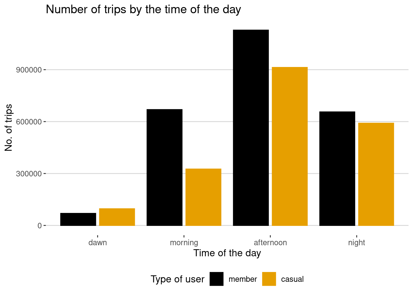
Regarding the time of day, it can be observed that the peak occurs at 17, 18 and 16 hours. The races decrease from afternoon, night, morning, until dawn.
-
Regarding to the month and season, the values decrease from summer, spring, autumn to winter. With the busiest months being June, August and July and the least busy months being February, December and January;
-
Regarding to the duration of the trip, the average duration is 26 minutes.
-
options(reactable.theme = reactableTheme(
  color = "hsl(233, 9%, 87%)",
  backgroundColor = "hsl(233, 9%, 19%)",
  borderColor = "hsl(233, 9%, 22%)",
  stripedColor = "hsl(233, 12%, 22%)",
  highlightColor = "hsl(233, 12%, 24%)",
  inputStyle = list(backgroundColor = "hsl(233, 9%, 25%)"),
  selectStyle = list(backgroundColor = "hsl(233, 9%, 25%)"),
  pageButtonHoverStyle = list(backgroundColor = "hsl(233, 9%, 25%)"),
  pageButtonActiveStyle = list(backgroundColor = "hsl(233, 9%, 28%)")
))


bikeshare_skim_member <- bikeshare_data |>
  group_by(member_casual) |>
  skimr::skim()


reactable(bikeshare_skim_member, filterable = TRUE, paginationType = "jump",
          columns = list(
  skim_type = colDef(
    cell = function(value) {
      htmltools::tags$b(value)
    }
  )
))
-
Regarding the difference in usage between members and casual users, we can observe the following:
-
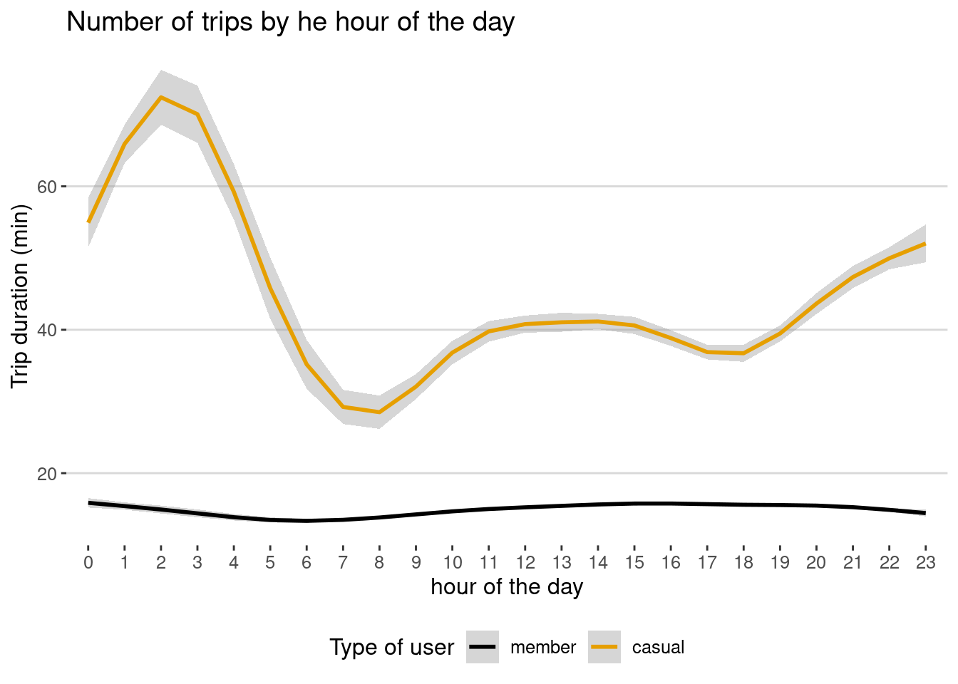
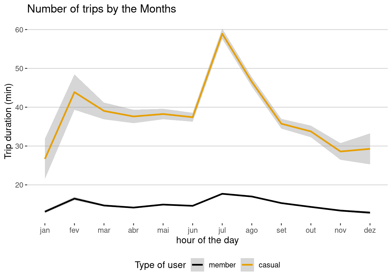
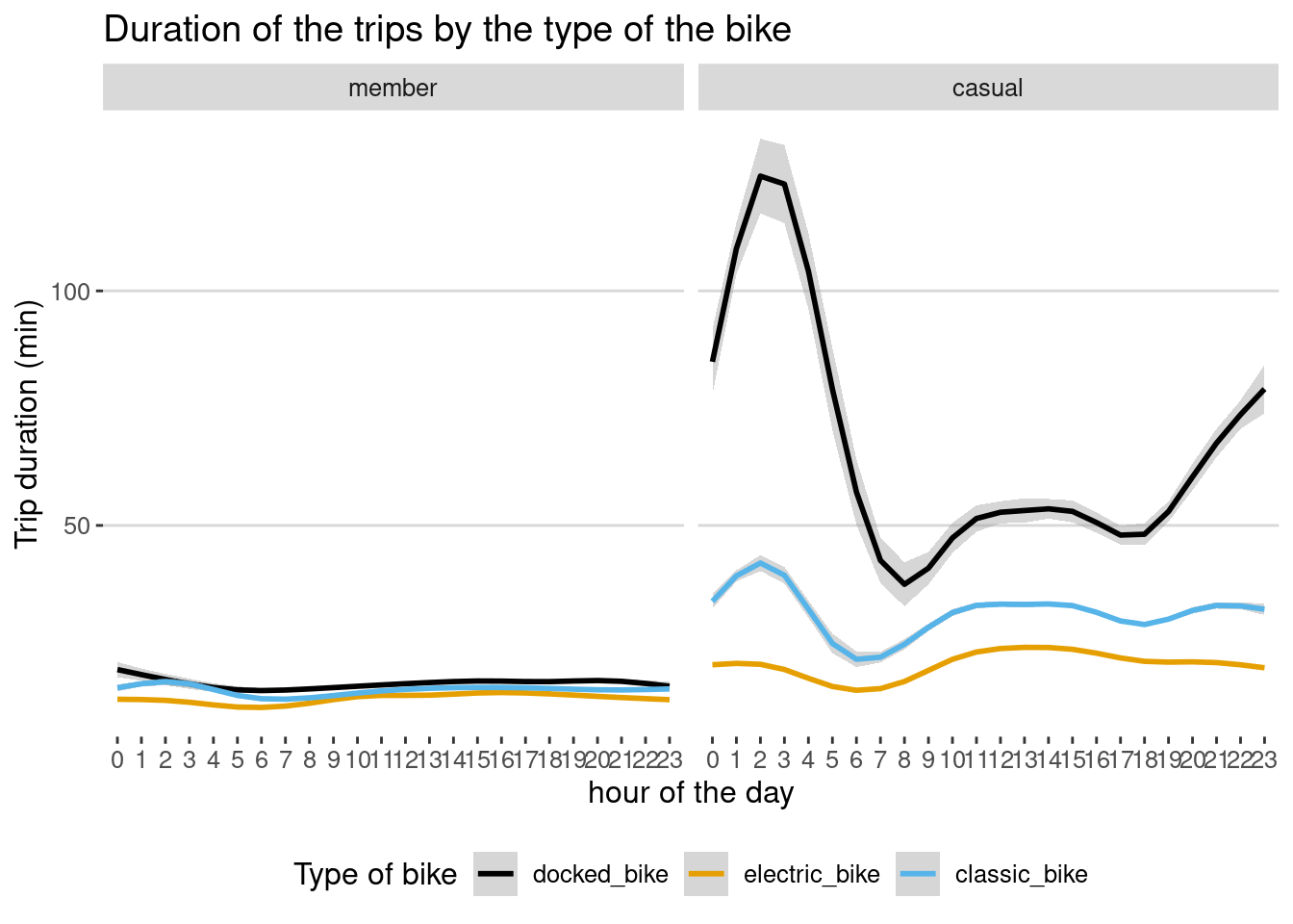
The trip duration is 170% longer for Casual Users. Averaging 40.1 min for casual users and 15.1 min for members;
-
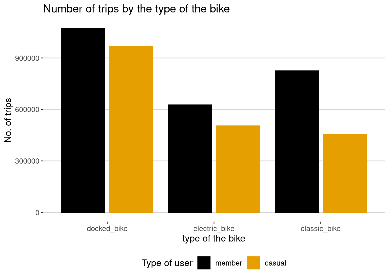
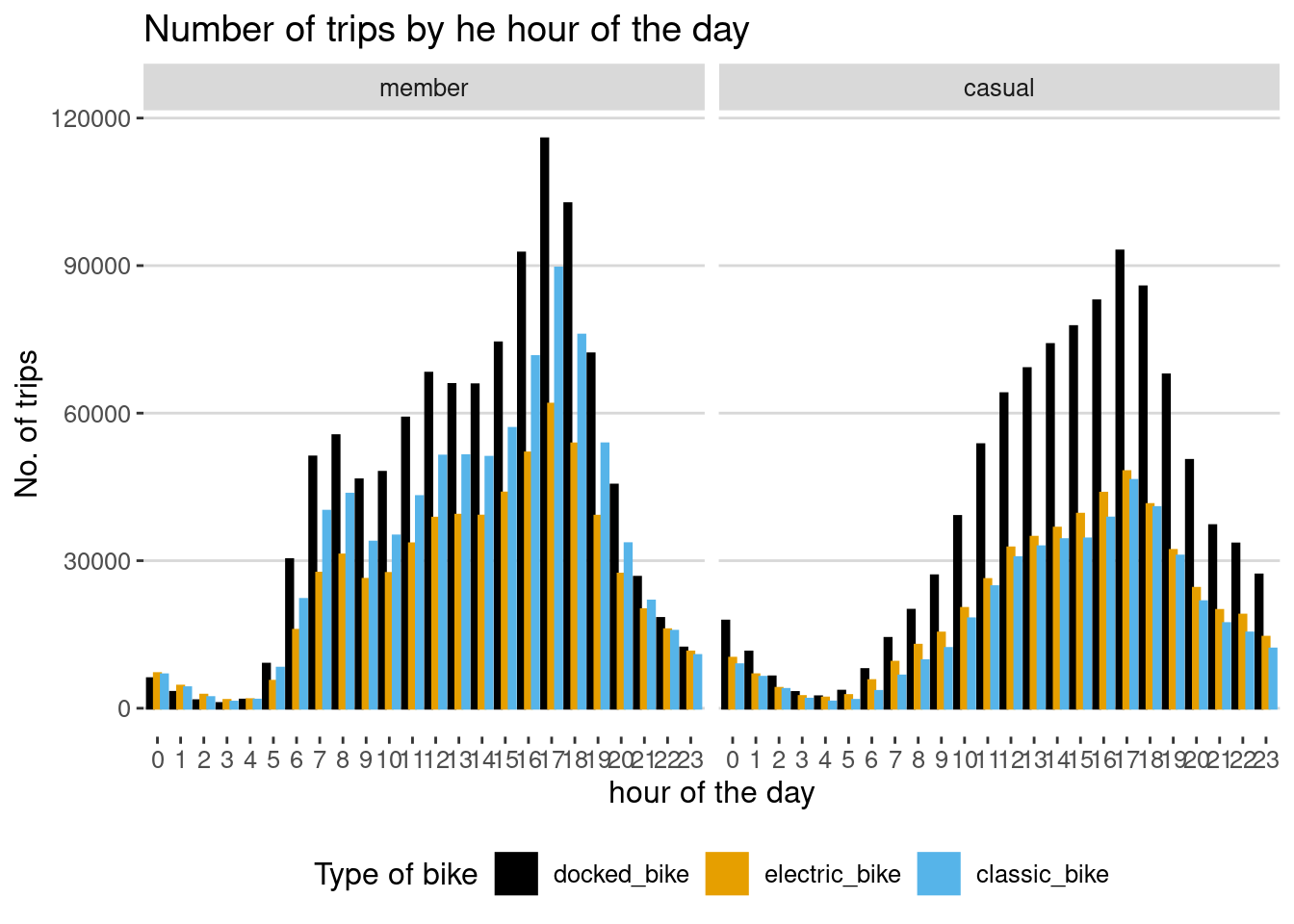
Regarding the type of bicycle, the most used for members, in descending order, are “docked”, “classic” and “eletric”. For casual users they are “docked”, “eletric” and “classic”;
-
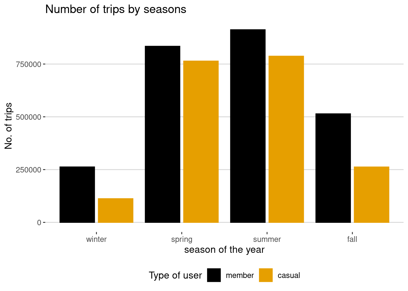
Regarding the time of year, both users follow the general average with a peak in summer and less use in winter;
-
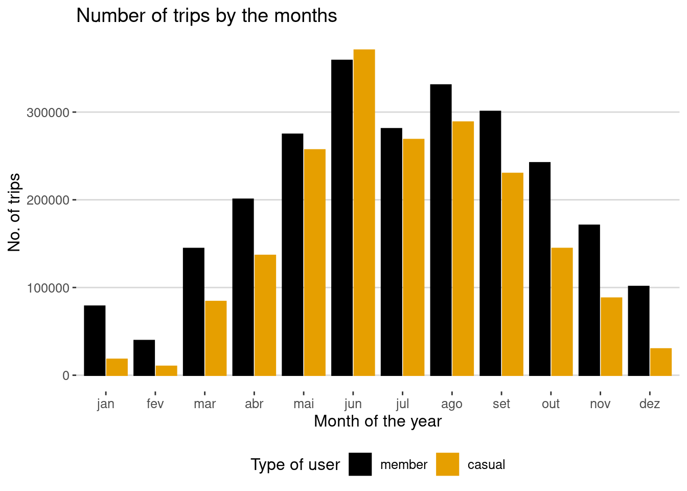
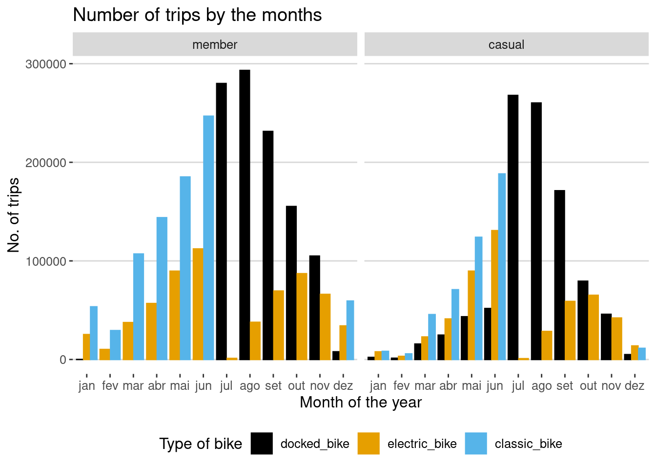
The busiest member months are June, August, September and July. For casual users, the busiest months are June, August, July and May;
-
Regarding the day of the week, the busiest days for members, in descending order, are Wednesday, Saturday, Friday and Tuesday. For casual users, the busiest days are Saturday, Sunday, Friday and Wednesday. With greater usage of the service on weekends for casual members compared to members;
-
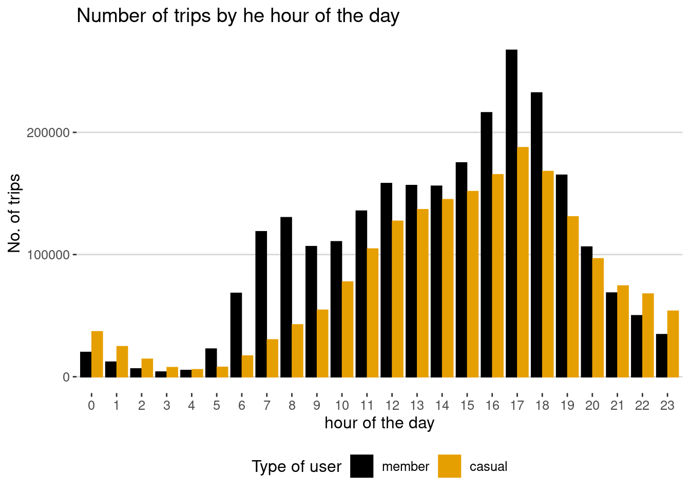
Regarding the time of day both types of users have more runs in the afternoon, however in casual members the night is busier than in the morning.
-
-
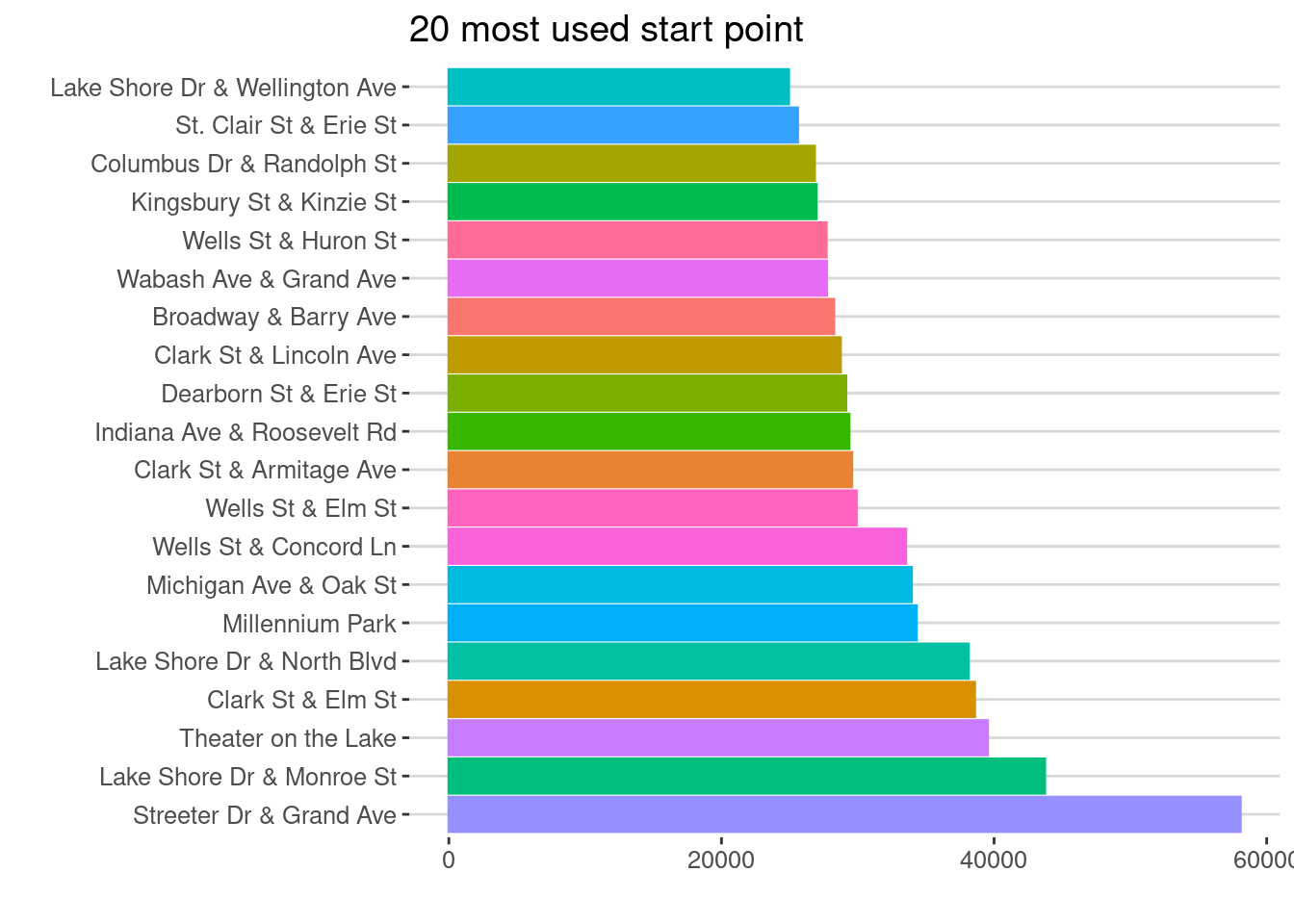
The Stations and routes more often used are the following:
bikeshare_data |>
  group_by(start_station_name) |>
  summarise(number_of_trips = n()) |>
  arrange(-number_of_trips) |>
  drop_na(start_station_name) |>
  slice(1:20)
# A tibble: 20 × 2
   start_station_name             number_of_trips
   <chr>                                    <int>
 1 Streeter Dr & Grand Ave                  58068
 2 Lake Shore Dr & Monroe St                43715
 3 Theater on the Lake                      39522
 4 Clark St & Elm St                        38576
 5 Lake Shore Dr & North Blvd               38115
 6 Millennium Park                          34304
 7 Michigan Ave & Oak St                    33945
 8 Wells St & Concord Ln                    33524
 9 Wells St & Elm St                        29896
10 Clark St & Armitage Ave                  29568
11 Indiana Ave & Roosevelt Rd               29365
12 Dearborn St & Erie St                    29132
13 Clark St & Lincoln Ave                   28735
14 Broadway & Barry Ave                     28245
15 Wabash Ave & Grand Ave                   27719
16 Wells St & Huron St                      27694
17 Kingsbury St & Kinzie St                 26953
18 Columbus Dr & Randolph St                26832
19 St. Clair St & Erie St                   25590
20 Lake Shore Dr & Wellington Ave           24929
bikeshare_data |>
  group_by(trip_route) |>
  summarise(number_of_trips = n()) |>
  arrange(-number_of_trips) |>
  drop_na(trip_route) |>
  slice(1:20)
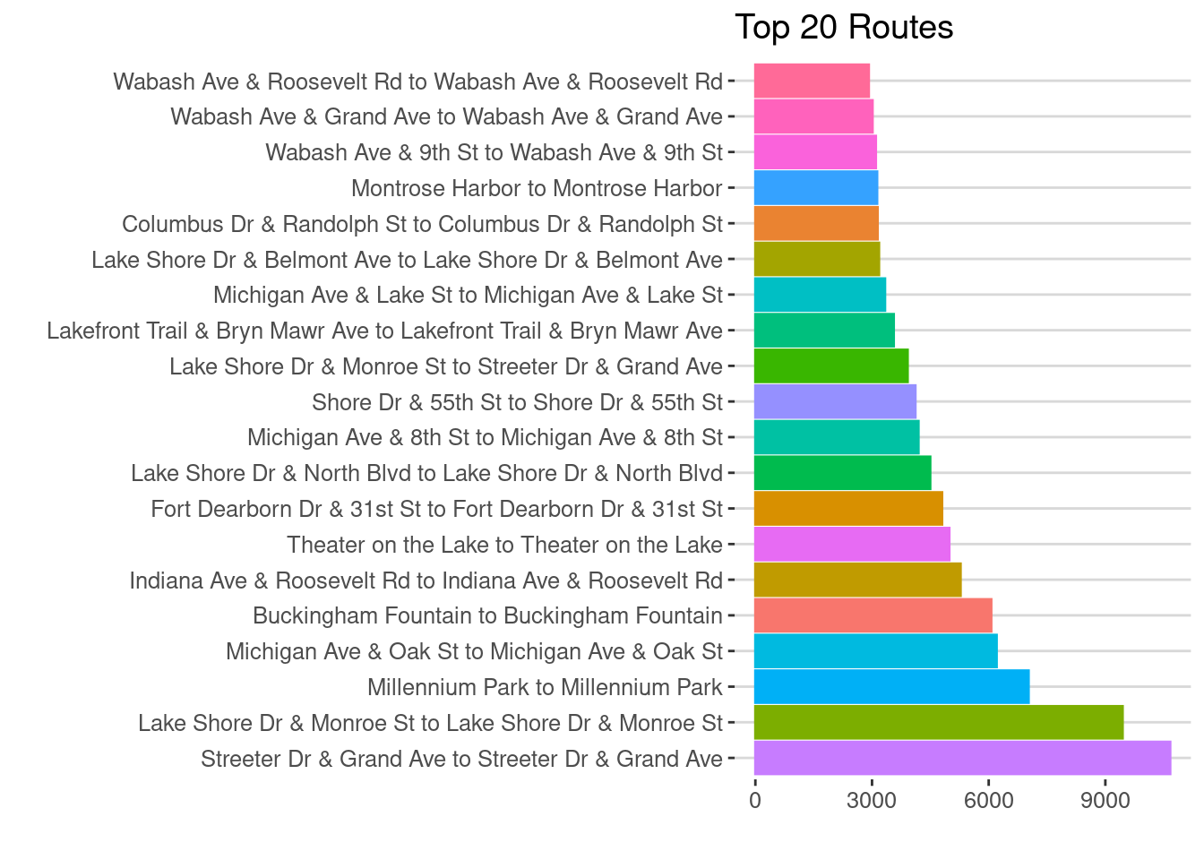
# A tibble: 20 × 2
   trip_route                                                    number_of_trips
   <chr>                                                                   <int>
 1 Streeter Dr & Grand Ave to Streeter Dr & Grand Ave                      10667
 2 Lake Shore Dr & Monroe St to Lake Shore Dr & Monroe St                   9443
 3 Millennium Park to Millennium Park                                       7025
 4 Michigan Ave & Oak St to Michigan Ave & Oak St                           6203
 5 Buckingham Fountain to Buckingham Fountain                               6065
 6 Indiana Ave & Roosevelt Rd to Indiana Ave & Roosevelt Rd                 5276
 7 Theater on the Lake to Theater on the Lake                               4986
 8 Fort Dearborn Dr & 31st St to Fort Dearborn Dr & 31st St                 4800
 9 Lake Shore Dr & North Blvd to Lake Shore Dr & North Blvd                 4495
10 Michigan Ave & 8th St to Michigan Ave & 8th St                           4193
11 Shore Dr & 55th St to Shore Dr & 55th St                                 4114
12 Lake Shore Dr & Monroe St to Streeter Dr & Grand Ave                     3914
13 Lakefront Trail & Bryn Mawr Ave to Lakefront Trail & Bryn Ma…            3557
14 Michigan Ave & Lake St to Michigan Ave & Lake St                         3333
15 Lake Shore Dr & Belmont Ave to Lake Shore Dr & Belmont Ave               3178
16 Columbus Dr & Randolph St to Columbus Dr & Randolph St                   3142
17 Montrose Harbor to Montrose Harbor                                       3130
18 Wabash Ave & 9th St to Wabash Ave & 9th St                               3097
19 Wabash Ave & Grand Ave to Wabash Ave & Grand Ave                         3012
20 Wabash Ave & Roosevelt Rd to Wabash Ave & Roosevelt Rd                   2916
Share Phase
By the hour and the time of the day
bikeshare_data |>
  group_by(member_casual, date_hour) |>
  summarise(n_trip = n(), .groups = 'drop') |>
  arrange(-n_trip) |>
  ggplot(mapping = aes(date_hour, n_trip)) +
  geom_col(aes(color = member_casual, fill = member_casual), position = "dodge2")+
  ggthemes::scale_color_colorblind()+
  ggthemes::scale_fill_colorblind()+
  scale_y_continuous(labels = function(x) format(x, scientific = FALSE))+
  ggthemes::theme_hc()+
  labs(
    title = "Number of trips by he hour of the day",
    color = "Type of user",
    fill = "Type of user",
    x = "hour of the day",
    y = "No. of trips"
    )
bikeshare_data |>
  group_by(member_casual, date_hour, trip_duration) |>
  ggplot(aes(x= date_hour, y = trip_duration, color = member_casual, group = member_casual)) +
  geom_smooth()+
  ggthemes::scale_color_colorblind()+
  ggthemes::scale_fill_colorblind()+
  ggthemes::theme_hc()+
  labs(
      title = "Number of trips by he hour of the day",
      color = "Type of user",
      fill = "Type of user",
      x = "hour of the day",
      y = "Trip duration (min)"
    )
bikeshare_data |>
  group_by(member_casual, day_time) |>
  summarise(n_trip = n(), .groups = 'drop') |>
  arrange(-n_trip) |>
  ggplot(mapping = aes(day_time, n_trip)) +
  geom_col(aes(color = member_casual, fill = member_casual), position = "dodge2")+
  ggthemes::scale_color_colorblind()+
  ggthemes::scale_fill_colorblind()+
  scale_y_continuous(labels = function(x) format(x, scientific = FALSE))+
  ggthemes::theme_hc()+
  labs(
      title = "Number of trips by the time of the day",
      color = "Type of user",
      fill = "Type of user",
      x = "Time of the day",
      y = "No. of trips"
    )
By Month and Season
bikeshare_data |>
  group_by(member_casual, date_month) |>
  summarise(n_trip = n(), .groups = 'drop') |>
  arrange(-n_trip) |>
  ggplot(mapping = aes(date_month, n_trip)) +
  geom_col(aes(color = member_casual, fill = member_casual), position = "dodge2")+
  ggthemes::scale_color_colorblind()+
  ggthemes::scale_fill_colorblind()+
  scale_y_continuous(labels = function(x) format(x, scientific = FALSE))+
  ggthemes::theme_hc()+
  labs(
      title = "Number of trips by the months",
      color = "Type of user",
      fill = "Type of user",
      x = "Month of the year",
      y = "No. of trips"
    )
bikeshare_data |>
  group_by(member_casual, date_month, trip_duration) |>
  ggplot(aes(x= date_month, y = trip_duration, color = member_casual, group = member_casual)) +
  geom_smooth()+
  ggthemes::scale_color_colorblind()+
  ggthemes::scale_fill_colorblind()+
  ggthemes::theme_hc()+
  labs(
      title = "Number of trips by the Months",
      color = "Type of user",
      fill = "Type of user",
      x = "hour of the day",
      y = "Trip duration (min)"
    )
bikeshare_data |>
  group_by(member_casual, date_season) |>
  summarise(n_trip = n(), .groups = 'drop') |>
  arrange(-n_trip) |>
  ggplot(mapping = aes(date_season, n_trip)) +
  geom_col(aes(color = member_casual, fill = member_casual), position = "dodge2")+
  ggthemes::scale_color_colorblind()+
  ggthemes::scale_fill_colorblind()+
  scale_y_continuous(labels = function(x) format(x, scientific = FALSE))+
  ggthemes::theme_hc()+
  labs(
      title = "Number of trips by seasons",
      color = "Type of user",
      fill = "Type of user",
      x = "season of the year",
      y = "No. of trips"
    )
By type of the bike
bikeshare_data |>
  group_by(member_casual, rideable_type) |>
  summarise(n_trip = n(), .groups = 'drop') |>
  arrange(-n_trip) |>
  ggplot(mapping = aes(rideable_type, n_trip)) +
  geom_col(aes(color = member_casual, fill = member_casual), position = "dodge2")+
  ggthemes::scale_color_colorblind()+
  ggthemes::scale_fill_colorblind()+
  scale_y_continuous(labels = function(x) format(x, scientific = FALSE))+
  ggthemes::theme_hc()+
  labs(
      title = "Number of trips by the type of the bike",
      color = "Type of user",
      fill = "Type of user",
      x = "type of the bike",
      y = "No. of trips"
    )
bikeshare_data |>
  group_by(member_casual, rideable_type, date_hour) |>
  summarise(n_trip = n(), .groups = 'drop') |>
  arrange(-n_trip) |>
  ggplot(mapping = aes(date_hour, n_trip)) +
  geom_col(aes(color = rideable_type, fill = rideable_type), position = "dodge2")+
  ggthemes::scale_color_colorblind()+
  ggthemes::scale_fill_colorblind()+
  scale_y_continuous(labels = function(x) format(x, scientific = FALSE))+
  ggthemes::theme_hc()+
  labs(
      title = "Number of trips by he hour of the day",
      color = "Type of bike",
      fill = "Type of bike",
      x = "hour of the day",
      y = "No. of trips"
    )+
  facet_wrap(vars(member_casual))
bikeshare_data |>
  group_by(member_casual, rideable_type, date_hour, trip_duration) |>
  ggplot(aes(x= date_hour, y = trip_duration, color = rideable_type, group = rideable_type)) +
  geom_smooth()+
  ggthemes::scale_color_colorblind()+
  ggthemes::scale_fill_colorblind()+
  ggthemes::theme_hc()+
  labs(
      title = "Duration of the trips by the type of the bike",
      color = "Type of bike",
      fill = "Type of bike",
      x = "hour of the day",
      y = "Trip duration (min)"
    )+
  facet_wrap(vars(member_casual))
bikeshare_data |>
  group_by(member_casual, rideable_type, date_month) |>
  summarise(n_trip = n(), .groups = 'drop') |>
  arrange(-n_trip) |>
  ggplot(mapping = aes(date_month, n_trip)) +
  geom_col(aes(color = rideable_type, fill = rideable_type), position = "dodge2")+
  ggthemes::scale_color_colorblind()+
  ggthemes::scale_fill_colorblind()+
  scale_y_continuous(labels = function(x) format(x, scientific = FALSE))+
  ggthemes::theme_hc()+
  labs(
      title = "Number of trips by the months",
      color = "Type of bike",
      fill = "Type of bike",
      x = "Month of the year",
      y = "No. of trips"
    )+
  facet_wrap(vars(member_casual))
Stations and the Routs more offen used
bikeshare_data |>
  group_by(start_station_name) |>
  summarise(n_trip = n()) |>
  arrange(-n_trip) |>
  drop_na(start_station_name) |>
  slice(1:20) |>
  ggplot(mapping = aes(fct_reorder(start_station_name, -n_trip), n_trip)) +
  geom_col(aes(color = start_station_name, fill = start_station_name), position = "dodge2")+
  coord_flip()+
  ggthemes::theme_hc()+
  theme(legend.position="none")+
  labs(
    title = "20 most used start point",
    x = "",
    y = ""
    )
bikeshare_data |>
  group_by(trip_route) |>
  summarise(n_trip = n()) |>
  arrange(-n_trip) |>
  drop_na(trip_route) |>
  slice(1:20) |>
  ggplot(mapping = aes(fct_reorder(trip_route, -n_trip), n_trip)) +
  geom_col(aes(color = trip_route, fill = trip_route), position = "dodge2")+
  coord_flip()+
  ggthemes::theme_hc()+
  theme(legend.position="none")+
  labs(
    title = "Top 20 Routes",
    x = "",
    y = ""
  )
Act
Key findings
- Different of members, casual user use service more often during the weekend;
- Also have the mean duration of the trips 170% higher than members;
- They the highest trip duration during dawn (from 12 am to 5 am) and at night (from 9 pm to 11 pm). With the pic at 2 am;
- During this time (from 9 pm to 3 am) the number of trips for casual users are higher than members;
- Casual users use the service mor from may to september;
- From june to september the have the highest trip duration in the year;
- use more eletrics bikes thans members.
Recommendations
- Create a subscription based on time-of-day to encourage casual users that ride from 9 pm to 5 am to subscribe;
- Implement discounts or a points system based on loyalty (frequency of use ) and high trip-duration users;
- Create seasonal subscriptions such as summer and spring. Or implement discounts on temporary subscriptions (3, 6, 9, 12 months);
- Create subscription especific to ride on week day or on the weekend;
- Create subscriptions for specific types of bicycles. Plans to use only electric bicycles, for example.